This page was generated from doc/euclidean/kochanek-bartels-uniform.ipynb. Interactive online version:

Uniform Kochanek–Bartels Splines§

As a starting point, remember the tangent vectors of uniform Catmull–Rom splines (see also equation 3 of [KB84]):

\begin{equation*} \boldsymbol{\dot{x}}_i = \frac{\boldsymbol{x}_{i+1} - \boldsymbol{x}_{i-1}}{2}, \end{equation*}

which can be re-written as

\begin{equation*} \boldsymbol{\dot{x}}_i = \frac{ (\boldsymbol{x}_i - \boldsymbol{x}_{i-1}) + (\boldsymbol{x}_{i+1} - \boldsymbol{x}_i) }{2}. \end{equation*}

Parameters§

TCB splines are all about inserting the parameters $T$, $C$ and $B$ into this equation.

Tension§

The usage of $T$ is shown in equation 4 of [KB84]:

\begin{equation*} \boldsymbol{\dot{x}}_i = (1 - T_i) \frac{ (\boldsymbol{x}_i - \boldsymbol{x}_{i-1}) + (\boldsymbol{x}_{i+1} - \boldsymbol{x}_i) }{2} \end{equation*}

Continuity§

Up to now, the goal was to have a continuous first derivative at the control points, i.e. the incoming and outgoing tangent vectors were identical:

\begin{equation*} \boldsymbol{\dot{x}}_i = \boldsymbol{\dot{x}}_i^{(-)} = \boldsymbol{\dot{x}}_i^{(+)} \end{equation*}

This also happens to be the requirement for a spline to be $C^1$ continuous.

The “continuity” parameter $C$ allows us to break this continuity if we so desire, leading to different incoming and outgoing tangent vectors (see equations 5 and 6 in [KB84]):

\begin{align*} \boldsymbol{\dot{x}}_i^{(-)} &= \frac{ (1 - C_i) (\boldsymbol{x}_i - \boldsymbol{x}_{i-1}) + (1 + C_i) (\boldsymbol{x}_{i+1} - \boldsymbol{x}_i) }{2}\\ \boldsymbol{\dot{x}}_i^{(+)} &= \frac{ (1 + C_i) (\boldsymbol{x}_i - \boldsymbol{x}_{i-1}) + (1 - C_i) (\boldsymbol{x}_{i+1} - \boldsymbol{x}_i) }{2} \end{align*}

Bias§

The usage of $B$ is shown in equation 7 of [KB84]:

\begin{equation*} \boldsymbol{\dot{x}}_i = \frac{ (1 + B_i) (\boldsymbol{x}_i - \boldsymbol{x}_{i-1}) + (1 - B_i) (\boldsymbol{x}_{i+1} - \boldsymbol{x}_i) }{2} \end{equation*}

All Three Combined§

To get the tangent vectors of a TCB spline, the three equations can be combined (see equations 8 and 9 in [KB84]):

\begin{align*} \boldsymbol{\dot{x}}_i^{(+)} &= \frac{ (1 - T_i) (1 + C_i) (1 + B_i) (\boldsymbol{x}_i - \boldsymbol{x}_{i-1}) + (1 - T_i) (1 - C_i) (1 - B_i) (\boldsymbol{x}_{i+1} - \boldsymbol{x}_i) }{2}\\ \boldsymbol{\dot{x}}_i^{(-)} &= \frac{ (1 - T_i) (1 - C_i) (1 + B_i) (\boldsymbol{x}_i - \boldsymbol{x}_{i-1}) + (1 - T_i) (1 + C_i) (1 - B_i) (\boldsymbol{x}_{i+1} - \boldsymbol{x}_i) }{2} \end{align*}

Note

There is an error in equation (6.11) of [Mil]. All subscripts of $x$ are wrong, most likely copy-pasted from the preceding equation.

To simplify the results we will get later, we introduce the following shorthands (as suggested in [Mil]):

\begin{align*} a_i &= (1 - T_i) (1 + C_i) (1 + B_i),\\ b_i &= (1 - T_i) (1 - C_i) (1 - B_i),\\ c_i &= (1 - T_i) (1 - C_i) (1 + B_i),\\ d_i &= (1 - T_i) (1 + C_i) (1 - B_i), \end{align*}

which lead to the simplified equations

\begin{align*} \boldsymbol{\dot{x}}_i^{(+)} &= \frac{ a_i (\boldsymbol{x}_i - \boldsymbol{x}_{i-1}) + b_i (\boldsymbol{x}_{i+1} - \boldsymbol{x}_i) }{2}\\ \boldsymbol{\dot{x}}_i^{(-)} &= \frac{ c_i (\boldsymbol{x}_i - \boldsymbol{x}_{i-i}) + d_i (\boldsymbol{x}_{i+1} - \boldsymbol{x}_i) }{2} \end{align*}

Calculation§

The tangent vectors are sufficient to implement Kochanek–Bartels splines (via Hermite splines). In the rest of this notebook we are deriving the basis matrix and the basis polynomials for comparison with other spline types.

[1]:

import sympy as sp
sp.init_printing()

As in previous notebooks, we are using some SymPy helper classes from utility.py:

[2]:

from utility import NamedExpression, NamedMatrix

And again, we are looking at the fifth spline segment from $\boldsymbol{x}_4$ to $\boldsymbol{x}_5$ (which can easily be generalized to arbitrary segments).

[3]:

x3, x4, x5, x6 = sp.symbols('xbm3:7')

[4]:

control_values_KB = sp.Matrix([x3, x4, x5, x6])
control_values_KB

[4]:

$\displaystyle \left[\begin{matrix}\boldsymbol{x}_{3}\\\boldsymbol{x}_{4}\\\boldsymbol{x}_{5}\\\boldsymbol{x}_{6}\end{matrix}\right]$

We need three additional parameters per vertex: $T$, $C$ and $B$. In our calculation, however, only the parameters belonging to $\boldsymbol{x}_4$ and $\boldsymbol{x}_5$ are relevant:

[5]:

T4, T5 = sp.symbols('T4 T5')
C4, C5 = sp.symbols('C4 C5')
B4, B5 = sp.symbols('B4 B5')

Using the shorthands mentioned above …

[6]:

a4 = NamedExpression('a4', (1 - T4) * (1 + C4) * (1 + B4))
b4 = NamedExpression('b4', (1 - T4) * (1 - C4) * (1 - B4))
c5 = NamedExpression('c5', (1 - T5) * (1 - C5) * (1 + B5))
d5 = NamedExpression('d5', (1 - T5) * (1 + C5) * (1 - B5))
display(a4, b4, c5, d5)

$\displaystyle a_{4} = \left(1 - T_{4}\right) \left(B_{4} + 1\right) \left(C_{4} + 1\right)$

$\displaystyle b_{4} = \left(1 - B_{4}\right) \left(1 - C_{4}\right) \left(1 - T_{4}\right)$

$\displaystyle c_{5} = \left(1 - C_{5}\right) \left(1 - T_{5}\right) \left(B_{5} + 1\right)$

$\displaystyle d_{5} = \left(1 - B_{5}\right) \left(1 - T_{5}\right) \left(C_{5} + 1\right)$

… we can define the tangent vectors:

[7]:

xd4 = NamedExpression(
    'xdotbm4^(+)',
    sp.S.Half * (a4.name * (x4 - x3) + b4.name * (x5 - x4)))
xd5 = NamedExpression(
    'xdotbm5^(-)',
    sp.S.Half * (c5.name * (x5 - x4)  + d5.name * (x6 - x5)))
display(xd4, xd5)

$\displaystyle \boldsymbol{\dot{x}}^{(+)}_{4} = \frac{a_{4} \left(- \boldsymbol{x}_{3} + \boldsymbol{x}_{4}\right)}{2} + \frac{b_{4} \left(- \boldsymbol{x}_{4} + \boldsymbol{x}_{5}\right)}{2}$

$\displaystyle \boldsymbol{\dot{x}}^{(-)}_{5} = \frac{c_{5} \left(- \boldsymbol{x}_{4} + \boldsymbol{x}_{5}\right)}{2} + \frac{d_{5} \left(- \boldsymbol{x}_{5} + \boldsymbol{x}_{6}\right)}{2}$

[8]:

display(xd4.subs_symbols(a4, b4))
display(xd5.subs_symbols(c5, d5))

$\displaystyle \boldsymbol{\dot{x}}^{(+)}_{4} = \frac{\left(1 - B_{4}\right) \left(1 - C_{4}\right) \left(1 - T_{4}\right) \left(- \boldsymbol{x}_{4} + \boldsymbol{x}_{5}\right)}{2} + \frac{\left(1 - T_{4}\right) \left(B_{4} + 1\right) \left(C_{4} + 1\right) \left(- \boldsymbol{x}_{3} + \boldsymbol{x}_{4}\right)}{2}$

$\displaystyle \boldsymbol{\dot{x}}^{(-)}_{5} = \frac{\left(1 - B_{5}\right) \left(1 - T_{5}\right) \left(C_{5} + 1\right) \left(- \boldsymbol{x}_{5} + \boldsymbol{x}_{6}\right)}{2} + \frac{\left(1 - C_{5}\right) \left(1 - T_{5}\right) \left(B_{5} + 1\right) \left(- \boldsymbol{x}_{4} + \boldsymbol{x}_{5}\right)}{2}$

Basis Matrix§

We try to find a transformation from the control values defined above to Hermite control values:

[9]:

control_values_H = sp.Matrix([x4, x5, xd4.name, xd5.name])
M_KBtoH = NamedMatrix(r'{M_{\text{KB$,4\to$H}}}', 4, 4)
NamedMatrix(control_values_H, M_KBtoH.name * control_values_KB)

[9]:

$\displaystyle \left[\begin{matrix}\boldsymbol{x}_{4}\\\boldsymbol{x}_{5}\\\boldsymbol{\dot{x}}^{(+)}_{4}\\\boldsymbol{\dot{x}}^{(-)}_{5}\end{matrix}\right] = {M_{\text{KB$,4\to$H}}} \left[\begin{matrix}\boldsymbol{x}_{3}\\\boldsymbol{x}_{4}\\\boldsymbol{x}_{5}\\\boldsymbol{x}_{6}\end{matrix}\right]$

If we substitute the above definitions of $\boldsymbol{\dot{x}}_4$ and $\boldsymbol{\dot{x}}_5$, we can obtain the matrix elements:

[10]:

M_KBtoH.expr = sp.Matrix([
    [expr.coeff(cv) for cv in control_values_KB]
    for expr in control_values_H.subs([xd4.args, xd5.args]).expand()])
M_KBtoH.pull_out(sp.S.Half)

[10]:

$\displaystyle {M_{\text{KB$,4\to$H}}} = \frac{1}{2} \left[\begin{matrix}0 & 2 & 0 & 0\\0 & 0 & 2 & 0\\- a_{4} & a_{4} - b_{4} & b_{4} & 0\\0 & - c_{5} & c_{5} - d_{5} & d_{5}\end{matrix}\right]$

Once we have a way to get Hermite control values, we can use the Hermite basis matrix from the notebook about uniform cubic Hermite splines …

[11]:

M_H = NamedMatrix(
    r'{M_\text{H}}',
    sp.Matrix([[ 2, -2,  1,  1],
               [-3,  3, -2, -1],
               [ 0,  0,  1,  0],
               [ 1,  0,  0,  0]]))
M_H

[11]:

$\displaystyle {M_\text{H}} = \left[\begin{matrix}2 & -2 & 1 & 1\\-3 & 3 & -2 & -1\\0 & 0 & 1 & 0\\1 & 0 & 0 & 0\end{matrix}\right]$

… to calculate the basis matrix for Kochanek–Bartels splines:

[12]:

M_KB = NamedMatrix(r'{M_{\text{KB},4}}', M_H.name * M_KBtoH.name)
M_KB

[12]:

$\displaystyle {M_{\text{KB},4}} = {M_\text{H}} {M_{\text{KB$,4\to$H}}}$

[13]:

M_KB = M_KB.subs_symbols(M_H, M_KBtoH).doit()
M_KB.pull_out(sp.S.Half)

[13]:

$\displaystyle {M_{\text{KB},4}} = \frac{1}{2} \left[\begin{matrix}- a_{4} & a_{4} - b_{4} - c_{5} + 4 & b_{4} + c_{5} - d_{5} - 4 & d_{5}\\2 a_{4} & - 2 a_{4} + 2 b_{4} + c_{5} - 6 & - 2 b_{4} - c_{5} + d_{5} + 6 & - d_{5}\\- a_{4} & a_{4} - b_{4} & b_{4} & 0\\0 & 2 & 0 & 0\end{matrix}\right]$

And for completeness’ sake, its inverse looks like this:

[14]:

M_KB.I

[14]:

$\displaystyle {M_{\text{KB},4}}^{-1} = \left[\begin{matrix}\frac{b_{4}}{a_{4}} & \frac{b_{4}}{a_{4}} & \frac{b_{4} - 2}{a_{4}} & 1\\0 & 0 & 0 & 1\\1 & 1 & 1 & 1\\\frac{- c_{5} + d_{5} + 6}{d_{5}} & \frac{- c_{5} + d_{5} + 4}{d_{5}} & \frac{- c_{5} + d_{5} + 2}{d_{5}} & 1\end{matrix}\right]$

Basis Polynomials§

[15]:

t = sp.symbols('t')

Multiplication with the monomial basis leads to the basis functions:

[16]:

b_KB = NamedMatrix(
    r'{b_{\text{KB},4}}',
    sp.Matrix([t**3, t**2, t, 1]).T * M_KB.expr)
b_KB.T.pull_out(sp.S.Half)

[16]:

$\displaystyle {b_{\text{KB},4}}^{T} = \frac{1}{2} \left[\begin{matrix}a_{4} t \left(- t^{2} + 2 t - 1\right)\\t^{3} \left(a_{4} - b_{4} - c_{5} + 4\right) + t^{2} \left(- 2 a_{4} + 2 b_{4} + c_{5} - 6\right) + t \left(a_{4} - b_{4}\right) + 2\\t \left(b_{4} + t^{2} \left(b_{4} + c_{5} - d_{5} - 4\right) + t \left(- 2 b_{4} - c_{5} + d_{5} + 6\right)\right)\\d_{5} t^{2} \left(t - 1\right)\end{matrix}\right]$

To be able to plot the basis functions, let’s substitute $a_4$, $b_4$, $c_5$ and $d_5$ back in (which isn’t pretty):

[17]:

b_KB = b_KB.subs_symbols(a4, b4, c5, d5).simplify()
b_KB.T.pull_out(sp.S.Half)

[17]:

$\displaystyle {b_{\text{KB},4}}^{T} = \frac{1}{2} \left[\begin{matrix}t \left(B_{4} + 1\right) \left(C_{4} + 1\right) \left(T_{4} - 1\right) \left(t^{2} - 2 t + 1\right)\\t^{3} \left(\left(B_{4} - 1\right) \left(C_{4} - 1\right) \left(T_{4} - 1\right) - \left(B_{4} + 1\right) \left(C_{4} + 1\right) \left(T_{4} - 1\right) - \left(B_{5} + 1\right) \left(C_{5} - 1\right) \left(T_{5} - 1\right) + 4\right) + t^{2} \left(- 2 \left(B_{4} - 1\right) \left(C_{4} - 1\right) \left(T_{4} - 1\right) + 2 \left(B_{4} + 1\right) \left(C_{4} + 1\right) \left(T_{4} - 1\right) + \left(B_{5} + 1\right) \left(C_{5} - 1\right) \left(T_{5} - 1\right) - 6\right) + t \left(T_{4} - 1\right) \left(\left(B_{4} - 1\right) \left(C_{4} - 1\right) - \left(B_{4} + 1\right) \left(C_{4} + 1\right)\right) + 2\\- t \left(t^{2} \left(\left(B_{4} - 1\right) \left(C_{4} - 1\right) \left(T_{4} - 1\right) + \left(B_{5} - 1\right) \left(C_{5} + 1\right) \left(T_{5} - 1\right) - \left(B_{5} + 1\right) \left(C_{5} - 1\right) \left(T_{5} - 1\right) + 4\right) - t \left(2 \left(B_{4} - 1\right) \left(C_{4} - 1\right) \left(T_{4} - 1\right) + \left(B_{5} - 1\right) \left(C_{5} + 1\right) \left(T_{5} - 1\right) - \left(B_{5} + 1\right) \left(C_{5} - 1\right) \left(T_{5} - 1\right) + 6\right) + \left(B_{4} - 1\right) \left(C_{4} - 1\right) \left(T_{4} - 1\right)\right)\\t^{2} \left(B_{5} - 1\right) \left(C_{5} + 1\right) \left(T_{5} - 1\right) \left(t - 1\right)\end{matrix}\right]$

Let’s use a helper function from helper.py:

[18]:

from helper import plot_basis

[19]:

labels = sp.symbols('xbm_i-1 xbm_i xbm_i+1 xbm_i+2')

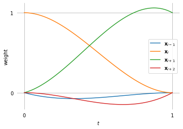
To be able to plot the basis functions, we have to choose some concrete TCB values.

[20]:

plot_basis(
    *b_KB.expr.subs({T4: 0, T5: 0, C4: 0, C5: 1, B4: 0, B5: 0}),
    labels=labels)

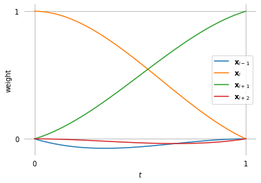
../_images/euclidean_kochanek-bartels-uniform_48_0.png

[21]:

plot_basis(
    *b_KB.expr.subs({T4: 0, T5: 0, C4: 0, C5: -0.5, B4: 0, B5: 0}),
    labels=labels)

../_images/euclidean_kochanek-bartels-uniform_49_0.png

Setting all TCB values to zero leads to the basis polynomials of uniform Catmull–Rom splines.