This page was generated from doc/euclidean/polynomials.ipynb. Interactive online version: .

Polynomial Parametric Curves

The building blocks for polynomial splines are of course polynomials.

import sympy as sp
sp.init_printing(order='grevlex')

We are mostly interested in univariate splines, i.e. curves with one free parameter, which are built using polynomials with a single parameter.

Here we are calling this parameter \(t\). You can think about it as time (e.g. in seconds), but it doesn’t have to represent time.

t = sp.symbols('t')

Polynomials typically consist of multiple terms. Each term contains a basis function, which itself contains one or more integer powers of \(t\). The highest power of all terms is called the degree of the polynomial.

The arguably simplest set of basis functions is the monomial basis, which simply consists of all powers of \(t\) up to the given degree:

b_monomial = sp.Matrix([t**3, t**2, t, 1]).T
b_monomial

$\displaystyle \left[\begin{matrix}t^{3} & t^{2} & t & 1\end{matrix}\right]$

In this example we are using polynomials of degree 3, which are also called cubic polynomials.

These basis functions are multiplied by (constant) coefficients. We are writing the coefficients with bold symbols, because apart from simple scalars (for one-dimensional functions), these symbols can also represent vectors in two- or three-dimensional space.

coefficients = sp.Matrix(sp.symbols('a:dbm')[::-1])
coefficients

$\displaystyle \left[\begin{matrix}\boldsymbol{d}\\\boldsymbol{c}\\\boldsymbol{b}\\\boldsymbol{a}\end{matrix}\right]$

We can create a polynomial by multiplying the basis functions with the coefficients and then adding all terms:

b_monomial.dot(coefficients)

$\displaystyle \boldsymbol{d} t^{3} + \boldsymbol{c} t^{2} + \boldsymbol{b} t + \boldsymbol{a}$

This is a cubic polynomial in its canonical form (because it uses monomial basis functions).

Let’s take a closer look at those basis functions (with some help from helper.py):

from helper import plot_basis

plot_basis(*b_monomial)

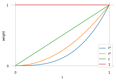
It doesn’t look like much, but every conceivable cubic polynomial can be formulated as exactly one linear combination of those basis functions (i.e. using one specific list of coefficients).

An example polynomial that’s not in canonical form …

example_polynomial = (2 * t - 1)**3 + (t + 1)**2 - 6 * t + 1
example_polynomial

$\displaystyle \left(2 t - 1\right)^{3} + \left(t + 1\right)^{2} - 6 t + 1$

from helper import plot_sympy, grid_lines

plot_sympy(example_polynomial, (t, 0, 1))
grid_lines([0, 1], [0, 0.5, 1])

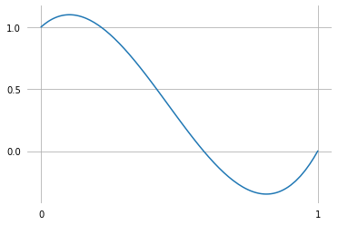
… can simply be re-written with monomial basis functions:

example_polynomial.expand()

$\displaystyle 8 t^{3} - 11 t^{2} + 2 t + 1$

Any polynomial can be rewritten using any set of basis functions (of appropriate degree).

In later sections we will see more basis functions, for example those that are used for Hermite, Bézier and Catmull–Rom splines.

In the previous example, we have used scalar coefficients to create a one-dimensional polynomial. We can use two-dimensional coefficients to create two-dimensional polynomial curves. Let’s create a little class to try this:

import numpy as np

class CubicPolynomial:

    grid = 0, 1

    def __init__(self, d, c, b, a):
        self.coeffs = d, c, b, a

    def evaluate(self, t):
        t = np.expand_dims(t, -1)
        return t**[3, 2, 1, 0] @ self.coeffs

Note

The @ operator is used here to do NumPy’s matrix multiplication.

Since this class has the same interface as the splines that will be discussed in later sections, we can use a spline helper function from helper.py for plotting:

from helper import plot_spline_2d

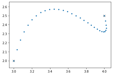
poly_2d = CubicPolynomial([-1.5, 5], [1.5, -8.5], [1, 4], [3, 2])

plot_spline_2d(poly_2d, dots_per_second=30, chords=False)

This class can also be used with three and more dimensions. The class splines.Monomial can be used to try this with arbitrary polynomial degree.