This page was generated from doc/euclidean/kochanek-bartels-properties.ipynb. Interactive online version: .

Properties of Kochanek–Bartels Splines

Kochanek–Bartels splines (a.k.a. TCB splines) are interpolating cubic polynomial splines, with three user-defined parameters per vertex (of course they can also be chosen to be the same three values for the whole spline), which can be used to change the shape and velocity of the spline.

These three parameters are called \(T\) for “tension”, \(C\) for “continuity” and \(B\) for “bias”. With the default values of \(C = 0\) and \(B = 0\), a Kochanek–Bartels spline is identical to a cardinal spline. If the “tension” parameter also has its default value \(T = 0\), it is also identical to a Catmull–Rom spline.

import splines

Let’s import a plotting function from helper.py …

from helper import plot_spline_2d

… and use it to implement a bespoke plotting function to illustrate the TCB parameters:

import matplotlib.pyplot as plt
import numpy as np

def plot_tcb(*tcb, ax=None):
    """Plot four TCB examples."""
    if ax is None:
        ax = plt.gca()
    vertices = [
        (-3.5, 0),
        (-1, 1.5),
        (0, 0.1),
        (1, 1.5),
        (3.5, 0),
        (1, -1.5),
        (0, -0.1),
        (-1, -1.5),
    ]
    for idx, tcb in zip([1, 7, 3, 5], tcb):
        all_tcb = np.zeros((len(vertices), 3))
        all_tcb[idx] = tcb
        s = splines.KochanekBartels(
            vertices, tcb=all_tcb, endconditions='closed')
        label = ', '.join(
            f'{name} = {value}'
            for name, value in zip('TCB', tcb)
            if value)
        plot_spline_2d(s, chords=False, label=label, ax=ax)
    plot_spline_2d(
        splines.KochanekBartels(vertices, endconditions='closed'),
        color='lightgrey', chords=False, ax=ax)
    lines = [l for l in ax.get_lines() if not l.get_label().startswith('_')]
    # https://matplotlib.org/tutorials/intermediate/legend_guide.html#multiple-legends-on-the-same-axes
    ax.add_artist(ax.legend(
        handles=lines[:2], bbox_to_anchor=(0, 0., 0.5, 1),
        loc='center', numpoints=3))
    ax.legend(
        handles=lines[2:], bbox_to_anchor=(0.5, 0., 0.5, 1),
        loc='center', numpoints=3)

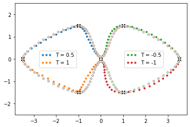
Tension

plot_tcb((0.5, 0, 0), (1, 0, 0), (-0.5, 0, 0), (-1, 0, 0))

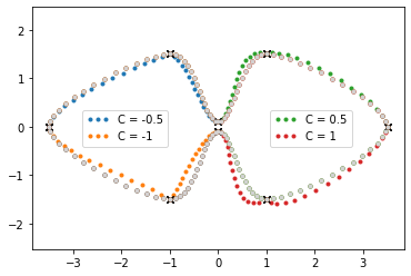
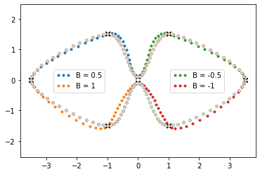
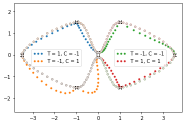
Continuity

plot_tcb((0, -0.5, 0), (0, -1, 0), (0, 0.5, 0), (0, 1, 0))

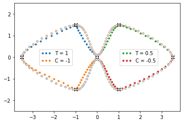
Note that the cases \(T = 1\) and \(C = -1\) have a very similar shape (a.k.a. “image”), but they have a different timing (and therefore different velocities):

plot_tcb((1, 0, 0), (0, -1, 0), (0.5, 0, 0), (0, -0.5, 0))

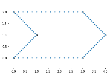
A value of \(C=-1\) on adjacent vertices leads to linear segments:

vertices1 = [(0, 0), (1, 1), (0, 2), (3, 2), (4, 1), (3, 0)]
s1 = splines.KochanekBartels(vertices1, tcb=(0, -1, 0), endconditions='closed')
plot_spline_2d(s1, chords=False)

Bias

This could also be called “overshoot” (if \(B > 0\)) and “undershoot” (if \(B < 0\)):

plot_tcb((0, 0, 0.5), (0, 0, 1), (0, 0, -0.5), (0, 0, -1))

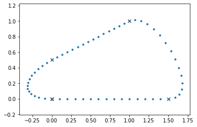
Bias \(-1\) followed by \(+1\) can be used to achieve linear segments between two control points:

vertices2 = [(0, 0), (1.5, 0), (1, 1), (0, 0.5)]
tcb2 = [(0, 0, -1), (0, 0, 1), (0, 0, -1), (0, 0, 1)]
s2 = splines.KochanekBartels(vertices2, tcb=tcb2, endconditions='closed')
plot_spline_2d(s2, chords=False)

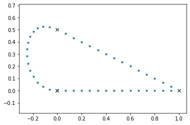
A sequence of \(B=-1\), \(C=-1\) and \(B=+1\) can be used to get two adjacent linear segments:

vertices3 = [(0, 0), (1, 0), (0, 0.5)]
tcb3 = [(0, 0, -1), (0, -1, 0), (0, 0, 1)]
s3 = splines.KochanekBartels(vertices3, tcb=tcb3, endconditions='closed')
plot_spline_2d(s3, chords=False)

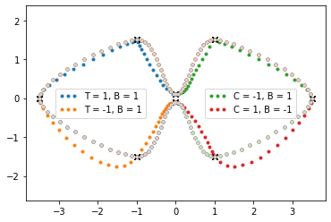
Combinations

plot_tcb((1, -1, 0), (-1, 1, 0), (-1, -1, 0), (1, 1, 0))

plot_tcb((1, 0, 1), (-1, 0, 1), (0, -1, 1), (0, 1, -1))