Barry–Goldman Algorithm With Slerp§
We can try to use the Barry–Goldman algorithm for non-uniform Euclidean Catmull–Rom splines using Slerp instead of linear interpolations, just as we have done with De Casteljau’s algorithm.
[1]:
def slerp(one, two, t):
"""Spherical Linear intERPolation."""
return (two * one.inverse())**t * one
[2]:
def barry_goldman(rotations, times, t):
"""Calculate a spline segment with the Barry-Goldman algorithm.
Four quaternions and the corresponding four time values
have to be specified. The resulting spline segment is located
between the second and third quaternion. The given time *t*
must be between the second and third time value.
"""
q0, q1, q2, q3 = rotations
t0, t1, t2, t3 = times
return slerp(
slerp(
slerp(q0, q1, (t - t0) / (t1 - t0)),
slerp(q1, q2, (t - t1) / (t2 - t1)),
(t - t0) / (t2 - t0)),
slerp(
slerp(q1, q2, (t - t1) / (t2 - t1)),
slerp(q2, q3, (t - t2) / (t3 - t2)),
(t - t1) / (t3 - t1)),
(t - t1) / (t2 - t1))
To illustrate this, let’s import NumPy and a few helpers from helper.py:
[3]:
import numpy as np
from helper import angles2quat, plot_rotation, plot_rotations
from helper import animate_rotations, display_animation
[4]:
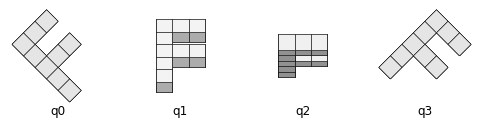
q0 = angles2quat(45, 0, 0)
q1 = angles2quat(0, -40, 0)
q2 = angles2quat(0, 70, 0)
q3 = angles2quat(-45, 0, 0)
[5]:
t0 = 0
t1 = 1
t2 = 5
t3 = 8
[6]:
plot_rotation({'q0': q0, 'q1': q1, 'q2': q2, 'q3': q3});
[7]:
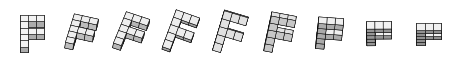
plot_rotations([
barry_goldman([q0, q1, q2, q3], [t0, t1, t2, t3], t)
for t in np.linspace(t1, t2, 9)
], figsize=(8, 1))
[8]:
ani = animate_rotations([
barry_goldman([q0, q1, q2, q3], [t0, t1, t2, t3], t)
for t in np.linspace(t1, t2, 50)
])
[9]:
display_animation(ani, default_mode='reflect')
For the next example, we use the splines.quaternion.BarryGoldman class:
[10]:
from splines.quaternion import BarryGoldman
[11]:
rotations = [
angles2quat(0, 0, 180),
angles2quat(0, 45, 90),
angles2quat(90, 45, 0),
angles2quat(90, 90, -90),
angles2quat(180, 0, -180),
angles2quat(-90, -45, 180),
]
[12]:
bg1 = BarryGoldman(rotations, alpha=0.5)
For comparison, we also create a Catmull–Rom-like quaternion spline using the class splines.quaternion.CatmullRom:
[13]:
from splines.quaternion import CatmullRom
[14]:
cr1 = CatmullRom(rotations, alpha=0.5, endconditions='closed')
[15]:
def evaluate(spline, frames=200):
times = np.linspace(
spline.grid[0], spline.grid[-1], frames, endpoint=False)
return spline.evaluate(times)
[16]:
ani = animate_rotations({
'Barry–Goldman': evaluate(bg1),
'Catmull–Rom-like': evaluate(cr1),
})
display_animation(ani, default_mode='loop')
Don’t worry if you don’t see any difference, the two are indeed extremely similar:
[17]:
0.0026694474661510537
However, when different time values are chosen, the difference between the two can become significantly bigger.
[18]:
grid = 0, 0.5, 1, 5, 6, 7, 10
[19]:
bg2 = BarryGoldman(rotations, grid)
cr2 = CatmullRom(rotations, grid, endconditions='closed')
[20]:
ani = animate_rotations({
'Barry–Goldman': evaluate(bg2),
'Catmull–Rom-like': evaluate(cr2),
})
display_animation(ani, default_mode='loop')
Constant Angular Speed§
A big advantage of de Casteljau’s algorithm is that when evaluating a spline at a given parameter value, it directly provides the appropriate tangent vector. When using the Barry–Goldman algorithm, the tangent vector has to be calculated separately, which make re-parameterization for constant angular speed very inefficient.
[21]:
class BarryGoldmanWithDerivative(BarryGoldman):
delta_t = 0.000001
def evaluate(self, t, n=0):
"""Evaluate quaternion or angular velocity."""
if not np.isscalar(t):
return np.array([self.evaluate(t, n) for t in t])
if n == 0:
return super().evaluate(t)
elif n == 1:
# NB: We move the interval around because
# we cannot access times before and after
# the first and last time, respectively.
fraction = (t - self.grid[0]) / (self.grid[-1] - self.grid[0])
before = super().evaluate(t - fraction * self.delta_t)
after = super().evaluate(t + (1 - fraction) * self.delta_t)
# NB: Double angle
return (after * before.inverse()).log_map() * 2 / self.delta_t
else:
raise ValueError('Unsupported n: {!r}'.format(n))
[22]:
from splines import ConstantSpeedAdapter
[23]:
bg3 = ConstantSpeedAdapter(BarryGoldmanWithDerivative(rotations, alpha=0.5))
Warning
Evaluating this spline takes a long time!
[24]:
%%time
bg3_evaluated = evaluate(bg3)
CPU times: user 1min 33s, sys: 17.7 ms, total: 1min 33s
Wall time: 1min 33s
[25]:
ani = animate_rotations({
'non-constant speed': evaluate(bg1),
'constant speed': bg3_evaluated,
})
[26]:
display_animation(ani, default_mode='loop')